
Contact Recycling
Contact recycling is a technique I developed for Box2D and Box3D. Contact recycling can drastically improve rigid body simulation performance, making the process of computing contact points almost free. Further, recycling can significantly improve stability.
Contact recycling combines ideas from other techniques. I had not seen this specific technique used in other physics engines as of March 2026 when I added it to Box2D in this pull request. There are similar solutions to the same problem but they have some fundamental differences. It is possible this specific technique already existed in some engines. Let me know and I’ll update this blog post.
Motivation
The motivation for contact recycling is straightforward. Often when there are many rigid bodies stacked together, there may be parts of the stack that are not moving much. Yet other parts of the stack are moving a lot and keeping the whole island awake. These stationary bodies should not have their contact points recomputed every time step. Can we devise a way to reuse the contact points from the previous time step? If so there can be massive performance gains because computing contact points is expensive. We should try to recycle them!
We can take this further. Consider a box resting on a train. Both are moving, but not relative to each other. These contact points should be recycled as well.
Before I explain contact recycling there is some background knowledge and terminology that is important to review.
Contact manifolds
A contact manifold is the surface of intersection between colliding convex shapes. A manifold for 2D collisions is a point or a line segment. A manifold for 3D collisions is a point, line segment, or a convex 2D polygon. Usually a line segment manifold will be represented by contact points at the endpoints. For a polygon manifold in 3D the contact points are at the vertices. In all cases the contact points all have the same normal vector, the manifold normal.
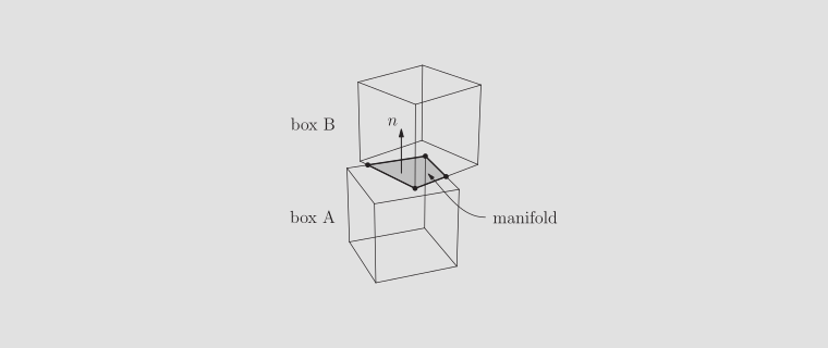 Contact Manifold
One-shot contact manifold
A one-shot contact manifold algorithm computes all the contact points for a manifold under one function call within one time step. Historically this implied using the Separating Axis Test (SAT) and Sutherland-Hodgman clipping. However, people have worked out how to do this with GJK by identifying convex hull features from the GJK simplex. GJK requires a fallback when there is overlap, such as SAT or the Expanding Polytope Algorithm (EPA).
Persistent contact manifold
Persistent contact manifold (PCM) algorithms seek to spread the work of building a contact manifold over several time steps. These are also called incremental manifolds. Early versions proceeded as follows:
- Compute closest points using GJK with EPA fallback
- Add the point from step 1 to the manifold
- Look for a point to remove from the manifold using some heuristic, such as:
- relative movement
- area contribution
- depth
Step 3 is necessary to keep the number of contact points small. According to the PhysX documentation, PCM improves performance but reduces stacking stability.
Avoiding computation
One-shot manifolds are clearly expensive. Even PCM requires a call to GJK every time step. GJK can be slow if the shapes are complex. By the way, I consider a 2D hull with over 8 points or a 3D hull with over 32 points to be complex.
The narrow phase can detect that the shapes or bodies haven’t moved much relative to each other and simply skip the manifold update and reuse the result from the previous step. Then it becomes a problem of finding a good heuristic for significant movement. For this, I’ll invoke an old friend.
Conservative Advancement
Conservative Advancement (CA) is traditionally a technique for continuous collision detection (CCD). The idea is to create an upper bound on the movement of two shapes relative to each other. Using this bound and the distance between the shapes, the CCD solver can iteratively move the bodies forward in time until they just touch or completely miss.
The premise of CA is that you can create a bound on the relative movement of two bodies (A and B) using:
$$(v_B - v_A) \cdot n + \|\omega_A\| h_A + \|\omega_B\| h_B$$Here \(n\) is the normal vector between the closest points, \(v\) is the linear velocity, and \(\omega\) is the angular velocity. The parameter \(h\) is the radius of the bounding circle centered on the center of mass (the rotation pivot). This is also called the maximum extent.
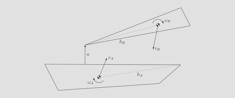 Conservative Advancement
This expression can be generally useful because it gives a way to combine linear and angular movement into a dimensionally consistent value. For example, Box2D uses this expression to measure the movement speed of a body for sleep and for CCD culling:
float maxVelocity = Length( v ) + Abs( omega ) * maxExtent;
Here maxExtent is the bounding radius of the body (\(h\) in the formula above). This formula gives the maximum velocity of any point on the body. I can compare this with the sleep threshold to determine if the body is sleepy. This is great because I don’t need a separate sleep threshold for angular velocity. This makes it so long skinny bodies don’t fall asleep too soon.
I can also compare maxVelocity to the inner circle of the smallest shape on the body to determine if the body is moving fast.
bool isFast = maxVelocity * timeStep > safetyFactor * minExtent;
Here minExtent is that inner radius and safetyFactor is some value between 0 and 1. If isFast == false then CCD can be skipped for this body. So one measure of speed can be used for two tests: sleepiness and speediness.
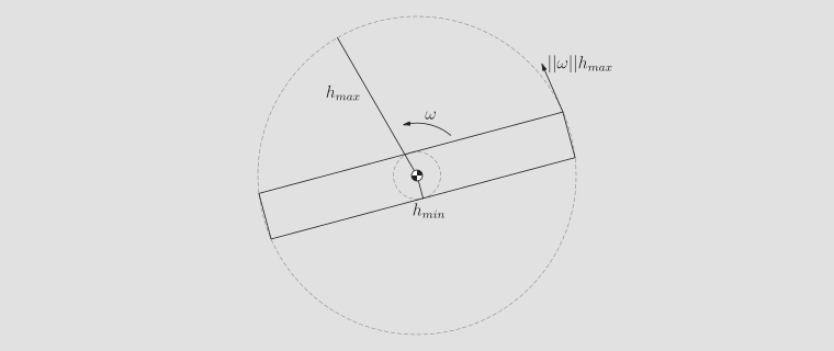 Extents
In the figure \(h_{max}\) is maxExtent and a \(h_{min}\) is minExtent.
Relative movement
The CA formula can be used for contact pairs to determine if the relative movement is significant. This gets conceptually tricky but the code is simple. Suppose we just computed a one-shot contact manifold. At this configuration we have the transform of the two bodies:
b2Transform cachedTransformA = bodyA->transform;
b2Transform cachedTransformB = bodyB->transform;
The relative transform is computed using the math library:
b2Transform cachedRelativeTransform = b2InvMulTransforms(cachedTransformA, cachedTransformB);
The order doesn’t matter. It just needs to be consistent. When there is a fresh contact I cache this relative transform and set a flag to indicate the transform has been cached. Then the next time step I compute the current relative transform.
b2Transform relativeTransform = b2InvMulTransforms(transformA, transformB);
Abbreviate the cached relative transform as xfc and the current transform as xf. With these I can compute the relative movement
of the bodies across the time step:
float relativeMovement = b2Distance(xfc.p, xf.p) + AngularDistance(xfc.q, xf.q) * maxExtent;
The AngularDistance function depends on how the rotations are represented. I take some shortcuts on this to avoid trigonometry. In Box2D
rotations are represented as cosine and sine pairs. I just use the absolute value of the sine term, which makes use of the small angle approximation:
I do something similar with quaternions in 3D except there is a factor of 2.
The maxExtent should be some combination of the two shape maximum extents. I use the maximum of the two extents but ignore extents of static bodies.
With all of that, I now have a single number, the relativeMovement, that indicates the frame over frame movement of the bodies relative to each other. If this is small enough then I can recycle the contacts.
A word of caution: do not update the cached relative transform when recycling. This causes drift. Only cache the relative transform on the step where the fresh manifold is computed.
Problem solved? Not quite. If you implement this you will find that you need a tight tolerance on the relative movement. If you loosen the tolerance then the simulation degrades quickly into a jitter fest. Do we give up? No, we evolve.
Updating separation
Box2D uses a solver I dub SoftStep. The idea is to use sub-steps instead of iterations and to use soft constraints to manage position error. So it uses soft sub-steps, or SoftStep for short. See the Solver2D post for details.
A key ingredient of the sub-stepping is to avoid recomputing contact points. Otherwise I might as well tell the user to use one iteration and small time steps. I make sub-stepping more efficient by reusing the contact points. For each sub-step I use the relative movement of the bodies and adjust the contact point separation value. This ensures shapes are pushed apart correctly. This is much cheaper than recomputing the contact points and leads to excellent stacking stability. Solver2D experiments showed that sub-stepping yields a better result than what can be achieved with a traditional iterative solver. Stacking and joints have increased stability.
I borrowed this idea of contact reuse across sub-steps with separation updates, and applied this to contact recycling across full time steps. When contact points are computed fresh I cache the initial separation values (baseSeparation). As the contact points are recycled, I adjust the current separation value by using the body transforms and the baseSeparation. Here’s the pseudocode:
// Contact recycling pseudocode. See Box2D/3D for full details.
if ( relativeMovement < tolerance )
{
    Rotation dqA = MultiplyRotations( qA, InvertRotation( cached_qA ) );
    Rotation dqB = MultiplyRotations( qB, InvertRotation( cached_qB ) );
    Vec2 normal = manifold.normal;
    Vec2 dc = centerB - centerA;

    for ( int i = 0; i < manifold.pointCount; ++i )
    {
        ManifoldPoint* mp = manifold.points + i;
        Vec2 rA = Rotate( dqA, mp->anchorA );
        Vec2 rB = Rotate( dqB, mp->anchorB );

        // Delta vector between the current contact points.
        Vec2 dp = dc + ( rB - rA );

        mp->separation = mp->baseSeparation + Dot( dp, normal );
    }
}
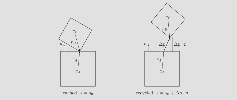 Separation Update
For the math to work out, I need to cache the rotations of both bodies, not just the relative transform. But the effect is glorious. Suddenly I can use very large tolerances, up to several centimeters. I observe increased stacking stability by recycling contact points this way. And that stability is greatly enhanced by updating the separation values.
As far as I know, this technique of updating the separation across time steps has not been done before. This may not seem like a big deal, but it makes a huge difference.
If you look closer at the code, you’ll see I hold the manifold normal in a fixed direction in world space. Also the contact anchors are fixed in world space. The anchors are rotated for the separation update, but those rotated anchor vectors are not preserved. The constraints apply impulses to the fixed anchors. These are the anchor vectors, not points. So the contact points translate with the bodies, but don’t rotate. This is the same as the sub-stepping strategy in Box2D.
It is tempting to use a local normal and anchor vectors, but they don’t work well in my experience, especially when considering rolling shapes, like circles. Ross Nordby (Bepu Physics) gave me the idea of keeping the anchor directions fixed. Holding the normal vector fixed goes back to the original release of Box2D. It just works better.
I recommend using a rotation tolerance with recycling to avoid a large error in the normal. If the bodies in contact are pinned together by some other constraint, then the simulation can break.
As with many things in game physics, the best way to understand the value is to see the behavior and performance in practice. So watch this video where I show how contact recycling works in practice and some of the artifacts it has when pushed too far. I also show the effect of updating the separation value.
Summary
Contact point reuse and separation update have been used for sub-stepping by multiple physics engines, including Bepu and PhysX. However, as far as I know, it has not been used across time steps with one-shot manifolds. It is straightforward to add contact recycling to a physics engine. The main requirements are:
- one-shot manifolds
- manifolds are cached
- anchor points coincide when the manifold is computed
The physics engine will achieve higher performance and stability with minimal structural changes. Having a sub-stepping solver is not required. I’m not sure contact recycling would work well with PCM because there could be conflicting heuristics. Maybe someone will try it.
References
Update
I originally wrote this post in May 2026, but the Box3D release pushed it aside.
Box2D/3D’s contact recycling has already been adopted by other physics engines.
Jondolf gives a kind attribution in his PR.