Solver2D
I was recently testing the Box2D version 3.0 alpha and found a stability problem. I found a fix for the problem fairly quickly, however the experience left me thinking about the progression of v3.0 and how the engine has been getting more features and more complexity. There are several joint types now. There is island management, multithreading, SIMD, graph coloring, continuous collision, and so on. These are all important features, but there is a problem.
Early in v3.0 development, I tested several solver variations. However, once I found a good solver, I removed the other solvers and the flexibility to try different solvers was gone. With all the new features and complexity of v3.0, it is no longer easy to try a new solver variation. I love tinkering with solvers, so I decided to create a new, simplified engine purely for the purpose of trying multiple different solvers. Thus Solver2D was born.
This code is a cut of Box2D version v3.0 with many features removed. No sleeping, only two joint types, no continuous collision, no threading, no graph coloring. The engine is designed to make trying different solvers as easy as possible with no extraneous features. I even removed profiling and timers.
The goal of Solver2D is to have a platform for testing, comparing, and developing as many solvers as I can. If I have an idea for a new solver, I can easily try it without messing up Box2D and I have all the collision, broad-phase, and UI stuff I need.
Inspiration
Once I committed to writing a framework for testing various solvers I began to draw inspiration from the game physics community. I knew I wanted to test and compare various solvers.
The Physics Engine Evaluation Lab (PEEL) by Pierre Terdiman is able run multiple physics engines simultaneously and show the results together in real-time. The image below shows PhysX and Jolt running the same simulation simultaneously in PEEL. Very cool!
 PEEL running PhysX and Jolt
PEEL is concerned with behavior, stability, performance, and creating fun demos. For Solver2D, I’m mainly concerned with comparing solver behavior and stability. I’ve left out performance considerations because that creates a lot of the complexity that I had just removed. Performance is certainly important, but that is just another axis of physics engine development. It is easily possible to have a slow and fast version of the exact same solver. On the other hand, I’m onboard with making fun demos!
I’ve also been inspired by the work on Position Based Dynamics (PBS) and in particular the application to rigid bodies within Extended Position Based Dynamics (XPBD). Solver2D gave me the opportunity to try out this solver.
Many Solvers
So far in Solver2D I have implemented 8 solvers! These are all Gauss-Seidel based solvers that attempt to solve constraints iteratively. Here’s the list of solvers:
- PGS (Baumgarte)
- PGS_NGS
- PGS_NGS_Block
- PGS_Soft
- TGS_Sticky (Baumgarte)
- TGS_Soft
- TGS_NGS
- XPBD
That’s a lot of acronyms! I’ll describe all the acronyms then I’ll describe each solver and what makes it unique.
Projected Gauss-Seidel (PGS)
PGS is the classic iterative method for solving constraints in game physics. I describe it in detail in Iterative Dynamics with Temporal Coherence. I implemented this method in the game Tomb Raider: Legend. This was in the days of the Playstation 2 when game consoles started to have some reasonable computational power.
Later I reframed PGS as Sequential Impulses. I believe this is an easier way to conceptualize and implement a game physics engine. And this lead to the creation of Box2D.
It turns out there are many variations of PGS. Some important concepts that are relevant to all PGS solvers:
- warm starting : feeding the impulses/forces of previous time steps to the next time step. The hope is to amortize the solution over several time steps, especially when objects are coming to a rest.
- accumulated impulse : we need to clamp impulses for one-way constraints like contact or limited constraints like friction. When we clamp the impulse, we should clamp the total impulse, not the impulse computed for the current iteration. This lets incremental impulses decrease the total impulse. This is crucial to avoid jitter.
- iteration count : solvers generally use a fixed number of iterations. The number is generally determined offline. In game physics there are typically 4 to 8 iterations.
In code, PGS looks like this:
float incrementalImpulse = -effectiveMass * relativeNormalVelocity;
float newAccumulatedImpulse = max(0.0f, accumulatedImpulse + incrementalImpulse);
float appliedImpulse = newAccumulatedImpulse - accumulatedImpulse;
accumulatedImpulse = newAccumulatedImpulse;
The effective mass depends on the mass properties and the location of the contact point relative to the center of mass of the two bodies. The relativeNormalVelocity is the relative velocity of the contact point on the two bodies projected onto the contact normal. There some logic clamp the accumulated impulse. Notice that the applied impulse will be the change in the accumulated impulse.
Temporal Gauss-Seidel (TGS)
TGS is an approach documented in the paper “Small Steps in Physics Simulation”. Yet the phrase Temporal Gauss-Seidel does not appear in the paper. Instead it comes from the documentation for the PhysX SDK.
This is probably good because TGS is a misnomer. Gauss-Seidel is numerical method for solving a linear system and Projected Gauss-Seidel is a method for solving a linear system with complementarity constraints. TGS doesn’t change this. Instead TGS refers to preferring sub-stepping over iteration.
Additionally, sub-stepping is not the most interesting part of TGS. It has long been known that smaller time steps are more effective than more iterations. This is based on the Taylor Series. As the step size gets smaller, the approximation improves and non-linearities fade away.
On the other hand what is interesting is the idea that we can do sub-stepping without updating the broad-phase or recomputing the contact points. It turns out with a little bit of vector algebra we can update contact points by storing them in local coordinates as this figure shows.
 contact updating during sub-stepping
We can track the contact point in both bodies across sub-steps. With that information we can update the separation value and push the bodies apart in response. Maintaining the same contact anchor points across sub-steps is approximate, but it turns out to work well. It would be very expensive to recompute the contact points every sub-step, so contact point updating has made sub-stepping a viable approach. Unfortunately this idea is not mentioned in the small steps paper.
// Compute the current contact separation for a sub-step
float separation = dot(pB + rB - pA - rA, normal) + originalSeparation;
Baumgarte Stabilization
Baumgarte Stabilization comes from a paper that sadly appears to be locked behind a paywall. Nevertheless the concept is simple: while solving constraints using impulses, boost the impulse a little bit to account for overlap and thus push the shapes apart.
Baumgarte Stabilization is simple to implement. It brings the current contact separation/overlap into the PGS impulse computation. It just changes one line:
float incrementalImpulse = -meff * (vn + 0.2f * contactSeparation / timeStep);
I’ve abbreviated the effective mass and relative normal velocity so that everything fits on one line. The value 0.2f is an arbitrary factor which is normally between 0 and 1. A value of 1 tries to resolve all overlap in a single time step while a factor of 0 has no effect.
This is a cheap, yet crude way to deal with overlap. The main complaint is that it is not physically accurate and it can lead to energy creation and jitter if not tuned carefully.
This is used in the PGS and TGS_Sticky solvers. Even though I’m not a fan of Baumgarte Stabilization, I think it is important to keep around for comparison.
Nonlinear Gauss-Seidel (NGS)
NGS emerged in the early days of Box2D as a way of dealing with the energetic response of Baumgarte Stabilization. The main idea is to solve position constraints after the velocity constraints. The position constraint solver looks a lot like the velocity constraint solver, but it uses pseudo velocities that don’t interact with the real velocities. This means that the position constraint solver doesn’t affect kinetic energy.
There can be a small amount of potential energy generation. It is not possible to resolve overlap without something moving, unless you want a physics engine that shrinks things when they start to overlap. Then we have a problem with mass conservation.
NGS is iterative like PGS, but instead of dealing with linear velocity constraints, it is dealing with non-linear position constraints. Position constraints are non-linear because they deal with rotations (sine/cosine/quaternions).
NGS deals with position impulses that are not influenced by the time step, which in turn makes NGS have behavior that is time step dependent overall. NGS looks like Baumgarte Stabilization with the relative normal velocity and the time step removed.
float positionImpulse = -effectiveMass * (0.2f * min(0.0f, contactSeparation));
It doesn’t make sense to accumulate or warm start the position impulses. At equilibrium the position impulse should be zero, so zero is always the best guess for the position impulse. This makes warm starting irrelevant. Accumulation can be problematic because it can lead to contacts pulling back. Instead, I just clamp the separation value.
In PGS the impulses are applied linearly to velocity like this:
linearVelocity += (appliedImpulse * normal) / mass;
angularVelocity += inverseInertiaTensor * cross(r, appliedImpulse * normal);
The value r is the vector from the center of mass to the contact point.
For NGS there is a position impulse that is applied to position and rotation:
position += (appliedImpulse * normal) / mass;
rotation = IntegrateRotation(rotation, inverseInertiaTensor * cross(r, apppliedImpulse * normal));
The position update is linear, but the rotation update is nonlinear. We need a special function IntegrateRotation that handles this. In Box2D version 2, I maintained the body angle directly, which looks linear until you see the resulting sine and cosine calls. In Solver2D I’m using a complex number with two components that represent the sine and cosine. The update for this is nonlinear as well because it involves a square root. This is the only thing that makes NGS nonlinear. Otherwise the math is identical to PGS.
NGS has been around a long time and I don’t think it is possible to attribute it to any one person or paper as far as I know.
Soft Constraints
Soft constraints have been around a long time, going back at least to ODE. I presented soft constraints at the GDC here.
I view soft constraints as an evolution of Baumgarte Stabilization. They are based on the harmonic oscillator, also known as the mass-spring-damper system. Like Baumgarte, a soft constraint can be used to push shapes apart and remove overlap. The advantage of soft constraints is they can dampen the response and soft constraints can be tuned intuitively by specifying the natural frequency in Hertz and the non-dimensional damping ratio.
Typically the Hertz is kept well below the time step. For example, we should keep the Hertz at 30Hz or below for a 60Hz time step. This is due to Nyquist’s Theorem.
Originally I thought of soft constraints as a nice way of simulating springs in the constraint solver. For example, in Tomb Raider, we used a soft weld (fixed) joint for the horizontal poles Lara would swing on. Those poles had a rotational frequency of just 1Hz or so and would flex as Lara would spin around them. However, with the introduction of sub-stepping (TGS), soft constraints have become more relevant.
With sub-stepping we are using smaller time steps, so we can use higher Hertz values for soft constraints, allowing them to appear more rigid. This is great because we can implement an efficient solver with a similar cost to Baumgarte Stabilization and much cheaper than NGS.
Recently I discovered that Ross Nordby of the Bepu physics engine had found a further simplification of the soft constraint parameters that makes them mass independent. Instead of two parameters that are coupled with body mass properties, he determined that you could use three parameters that are independent of the mass properties. Ross was able to express soft constraints with these three parameters that are computed using only the Hertz, damping ratio, and time step:
- bias rate
- mass coefficient
- impulse coefficient
Bepu also has a sub-stepping solver with contact separation updates and an advanced multithreading design. It is very fast! I recommend to check it out.
Here are the formulas for soft constraints:
float zeta = 1.0f; // damping ratio
float hertz = 5.0f; // cycles per second
float omega = 2.0f * pi * hertz; // angular frequency
float a1 = 2.0f * zeta + omega * timeStep;
float a2 = timeStep * omega * a1;
float a3 = 1.0f / (1.0f + a2);
float biasRate = omega / a1;
float massCoeff = a2 * a3;
float impulseCoeff = a3;
The bias rate has units of inverse time while the mass and impulse coefficients are non-dimensional.
The soft constraint is applied by modifying the PGS impulse:
float incrementalImpulse = -massCoeff * meff * (vn + biasRate * contactSeparation) - impulseCoeff * accumulatedImpulse;
Notice the presence of the accumulated impulse. The impulse coefficient causes the incremental impulse to be reduced as the total impulse becomes large.
Relaxation
Relaxation is another concept that is important for my recent solver experiments. When we apply Baumgarte Stabilization or soft constraints we may be adding some undesirable springiness to the constraints. The idea is to relax that extra energy in the velocities and constraint impulses. This doesn’t come for free, but it is quite simple to implement. Here is some pseudo code:
bool applyBias = true;
// Solve constraints and apply Baumgarte Stabilzation or the soft constraint spring and damper.
SolveConstraints(timeStep, applyBias);
IntegratePositions(timeStep);
applyBias = false;
// Solve the constraints again, but don't apply any form of stabilization or softness.
SolveConstraints(timeStep, applyBias);
With Baumgarte Stabilization or soft constraints, the first call to SolveConstraints will add extra energy to the impulses to push the bodies apart. Then I’m updating the body positions based on those energized velocities. However, in the second call to SolveConstraints I’m disabling the use of Baumgarte Stabilization or soft constraints. This serves to remove the extra energy from the velocities and constraint impulses. Also notice that the positions are not updated from these relaxed velocities. This is intentional.
Relaxation is expensive, but it improves the simulation quality dramatically. However, we should determine empirically how useful this is and that is yet another reason I created Solver2D.
Solver Overview
Now that I have defined all the acronyms and main concepts, let’s review the solvers that I have implemented! I will go through these in a somewhat chronological order, based on when they became known to me.
PGS
The PGS solver is essentially Box2D-Lite, which I created in 2006. It is the Sequential Impulse version of PGS. It uses warm starting and Baumgarte Stabilization. I consider this the minimum viable rigid body solver.
PGS_NGS
This is the PGS solver with a NGS position solver instead of Baumgarte Stabilization. This went into Box2D version 1.0 in 2007, back when Box2D was hosted on SourceForge! NGS was a nice feature in Box2D because it meant that objects that start with overlap do not fly apart, instead they are pushed apart gently.
PGS_NGS_Block
This is an evolution of PGS_NGS that adds a small direct solver for the Linear Complementarity Problem (LCP) for contacts. This solves two contact points simultaneously, leading to better stacking stability. This is expensive, but the cost may be worth it in some games. Otherwise this solver is identical to PGS_NGS. This solver was implemented in Box2D version 2.0.
PGS_Soft
This is the PGS solver with soft constraints rather than Baumgarte Stabilization. It also adds relaxation iterations.
TGS_Sticky
This is a TGS solver that uses sub-steps and no iteration. It uses Baumgarte Stabilization and relaxation, but no warm starting. What makes it special is that friction anchors are stored across whole time steps. Baumgarte Stabilization is applied to the friction anchors to pull them together tangentially. Friction anchors are reset if the friction forces exceed the Coulomb friction limit.
I think this is a very interesting solver because it achieves stable stacking with no warm starting of the impulses. The only warm starting is the friction anchors. This shows how important strong friction is to stable stacking. There are some artifacts and you may see tangential oscillations.
TGS_Soft
This is a TGS solver with the whole kitchen sink:
- sub-stepping instead of iterations
- warm starting
- soft constraints
- relaxation
It is basically PGS_Soft converted to sub-stepping. I plan to use this solver in Box2D version 3.
TGS_NGS
This is a conversion of PGS_NGS from iteration to pure sub-stepping.
XPBD
This is the Extended Position Base Dynamics rigid body solver I referenced above. This solver is much different than the other solvers, yet it was fairly simple to implement in Solver2D. It is somewhat like NGS without the PGS part. Unlike NGS, XPBD has been enhanced to handle friction and compute contact forces from positional corrections.
Some implementation details I had to infer. For example, I’m skipping the velocity projection if the normal impulse is zero (equation 35 in the associated paper). I had trouble getting friction to work well with XPBD as you can see in the samples. I may have made mistakes in my implementation, but I did spend quite some time going over things. Please file an issue if you find an error or something that should be improved.
Precision improvements
I made some samples that show behavior far from the origin. While I was doing this, I noticed XPBD had some serious problems. Not only was the simulation unstable, objects were actually floating. I realized this is due to code like this in XPBD:
body->linearVelocity = (body->position - body->position0) / timeStep;
Unlike other solvers, PBD derives velocity from positional changes. When an objects is very far from the origin, subtracting the old position from the new position may have a low number of significant digits, especially if the motion is slow. This can make bodies stop moving for even float.
I modified XPBD so that the solver operates on the change in position or deltaPosition. Then the velocity is computed as follows:
body->linearVelocity = body->deltaPosition / timeStep;
The absolute position isn’t touched until the end of the time step:
body->position = body->position0 + body->deltaPosition;
This fairly small change resolved the round-off errors I was seeing relative to other solvers. But why stop there? Sub-stepping and NGS have similar round-off issues as XPBD, so I converted all solvers to use deltaPosition. I also went through all the collision code to make sure contact points are computed and stored in local coordinates. I also created a lot of samples that show behavior far from the origin.
Object size at large coordinates is an important consideration. If your game has small objects far from the origin then accuracy will diminish faster than a game with large objects. So I added a 1 meter length scale indicator to the user interface. This image shows a pile of ragdolls over 30km from the origin. The bottom left of the screen shows a one meter horizontal line.
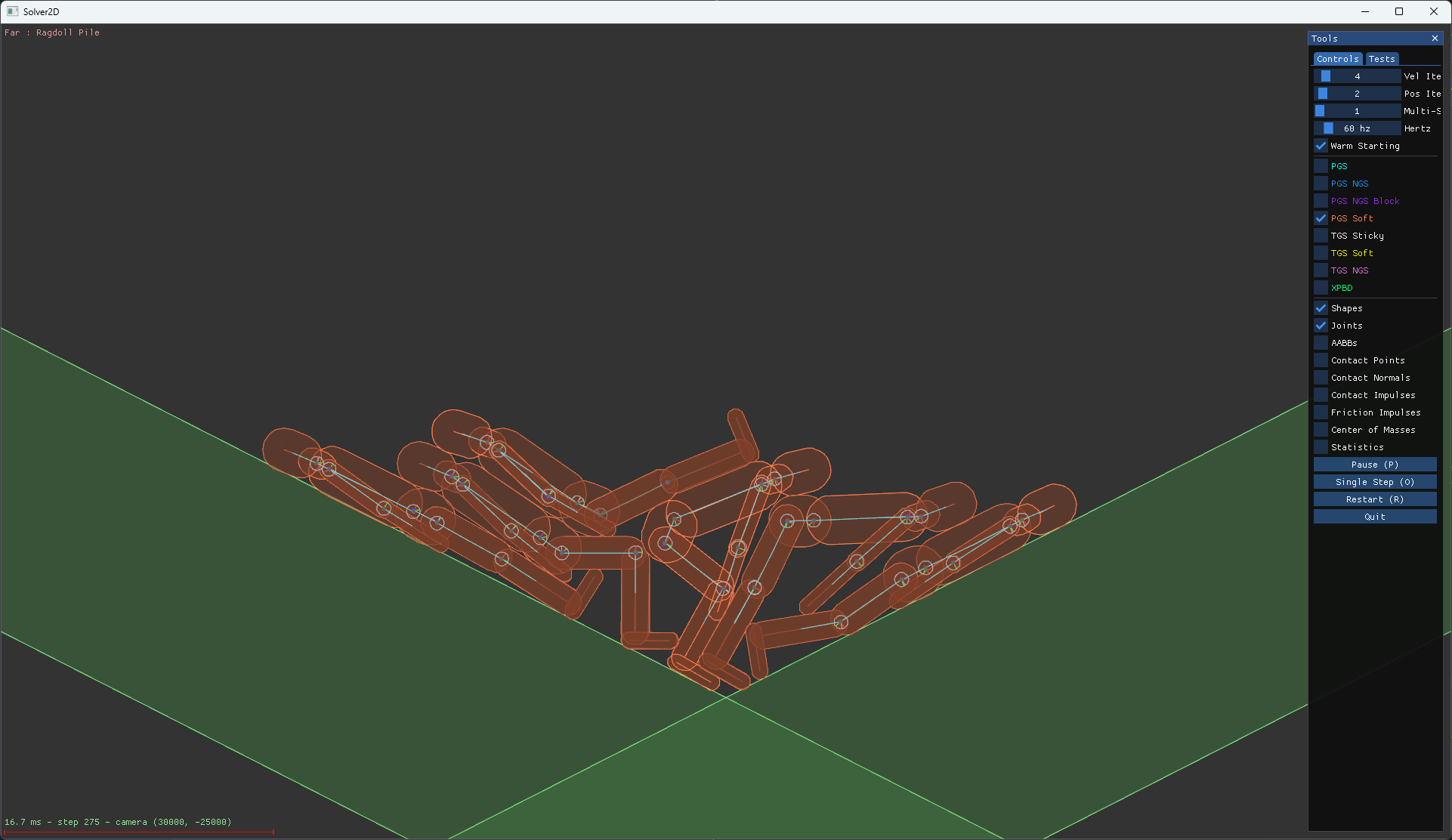 A pile of ragdolls over 30km from the origin
What about 3D?
When it comes to solver algorithms there is nothing substantially different between 2D and 3D. The thing that makes rigid body solvers challenging is rotation and this is present in both 2D and 3D. A solver that doesn’t work well in 2D will likely also not work well in 3D. In some ways, 2D is more demanding because the viewing angle shows overlap errors and/gaps more clearly. Furthermore, jitter can be more noticeable because objects don’t obscure each other in 2D.
This means that Solver2D is a good platform for developing and comparing solvers for both 2D and 3D applications. I’ve been developing 3D physics engines as part of my work and often I develop algorithms in 2D before I implement them in 3D. It is faster to develop the 2D version and easier to test.
Results
I created many samples that push these solvers to their limit. I’m testing large mass ratios, large coordinates, significant overlap, etc. I’ve also reduced the iteration count to a number lower than is typically used in games. Here is the setup for all samples:
- primary/velocity iterations : 4
- secondary/position iterations : 2
- simulation rate : 60 Hertz
For solvers with sub-stepping (TGS solvers), the primary iteration count corresponds to the number of sub-steps. Some solvers have secondary iterations: NGS has position iterations, PGS_Soft and TGS_Sticky have separate relax iterations.
Caveat: I’ve tuned all the solvers so they perform well on average across all samples. I am not tuning the solvers per sample. However, there may be tuning values I’ve overlooked and/or there may be bugs. This is why I’m making all this code open source. If you find a way to improve these solvers I will be happy to integrate those changes and update this post.
This videos shows the important samples and compares all the solvers.
Update: Performance
Solver2D is not optimized, so it is not appropriate to compare absolute performance numbers for all the solvers. However, I think it is meaningful to compare the number of body and constraint traversals each solver must perform for the 4/2 iteration limits. The actual number of traversals in Solver2D may be higher as these numbers account for loops that could be easily merged. For example, constraint preparation can often be merged with warm starting, but I didn’t write it that way in order to allow for more code sharing. There are some loops that could probably be merged with some extra effort, but that is not reflected in this table.
| Solver | Body Loops | Constraint Loops |
|---|---|---|
| PGS | 2 | 6 |
| PGS NGS | 3 | 8 |
| PGS NGS Block | 3 | 8 |
| PGS Soft | 3 | 8 |
| TGS Sticky | 11 | 8 |
| TGS Soft | 9 | 10 |
| TGS NGS | 9 | 10 |
| XPBD | 9 | 10 |
Constraint loops are much more expensive than body loops. Constraints do more math and they also have more cache misses when a constraint accesses the connected bodies. So if we want to compare solvers at a somewhat equal performance level, I would add more primary iterations to solvers with lower constraint loop counts to bring them up to par. Here’s what I suggest:
| Solver | Added Primary Iterations | Total |
|---|---|---|
| PGS | 4 | 8 |
| PGS NGS | 2 | 6 |
| PGS NGS Block | 2 | 6 |
| PGS Soft | 2 | 6 |
| TGS Sticky | 2 | 6 |
| TGS Soft | 0 | 4 |
| TGS NGS | 0 | 4 |
| XPBD | 0 | 4 |
Here’s the result for the large pyramid test:
Future
There are certainly more solver variations than I’ve tried so far. Here are some future options to try:
- Shock propagation, from the paper “Nonconvex Rigid Bodies with Stacking”
- Conjugate residual method, from the paper “Non-Smooth Newton Methods for Deformable Multi-Body Dynamics”
- A direct solver. I’m not sure what the state of the art is for direct solvers, so this would require more research.
- GPU friendly solvers. Jacobi, mass-splitting, etc.
I’ve also thought about adding a joint coordinate solver, like Featherstone’s algorithm. However, this is not a complete solver because it does not address contact. Still it might be interesting to see it for ragdolls and other samples with joints.
However, I should probably get back to finishing Box2D version 3.0!
Update 2
In the release of Box2D version 3.0 I’m now calling TGS Soft by the more appropriate name Soft Step (soft constraints + sub-stepping).
3909 words
2024-02-04 16:00 -0800