
Inscribed Spheres
The separating axis test (SAT) works well for computing contact manifolds. Unlike GJK, it is robust when shapes are very close together and it works when shapes are overlapped. Box3D uses SAT for computing the contact manifolds between convex hulls (polytopes). I like using SAT because I can get all the contact points at once and it doesn’t need a fallback algorithm for overlap like GJK does. So I don’t need to waste time calling GJK only to have it fail and then drop to a fallback algorithm like EPA or SAT. I also don’t need to shrink shapes to keep collision in the cheaper GJK regime.
SAT is expensive
SAT between polytopes can be quite expensive. If you are not careful it can become \(O(N^3)\) in the number of vertices. Most of the cost is testing edge pairs for separation. Box3D already has many different ways to speed up SAT between polytopes:
- The Gauss map is used to test edge pairs and reject them quickly when they don’t live on the surface of the Minkowski difference.
- Faces adjacent to an edge are used to avoid computing support points in the edge pair tests.
- SIMD is used to test four edge pairs at once.
- The narrow-phase caches feature pairs and re-uses them across time steps until a separation tolerance is exceeded.
- Contact recycling is used to completely skip the contact point computation when the relative motion between shapes is less than around 5cm. I update the separation values when a manifold is recycled to keep stacking stable.
As you can see, there is a lot of effort made to speed up SAT. Despite all that, Box3D can still be a bit slow when dealing with large piles of complex polytopes. The Convex Pile benchmark shows this. It is dominated by SAT. Namely the edge pair test is a hot loop that consumes many cycles. The feature cache and contact recycling don’t help much in the beginning when everything is moving quickly.
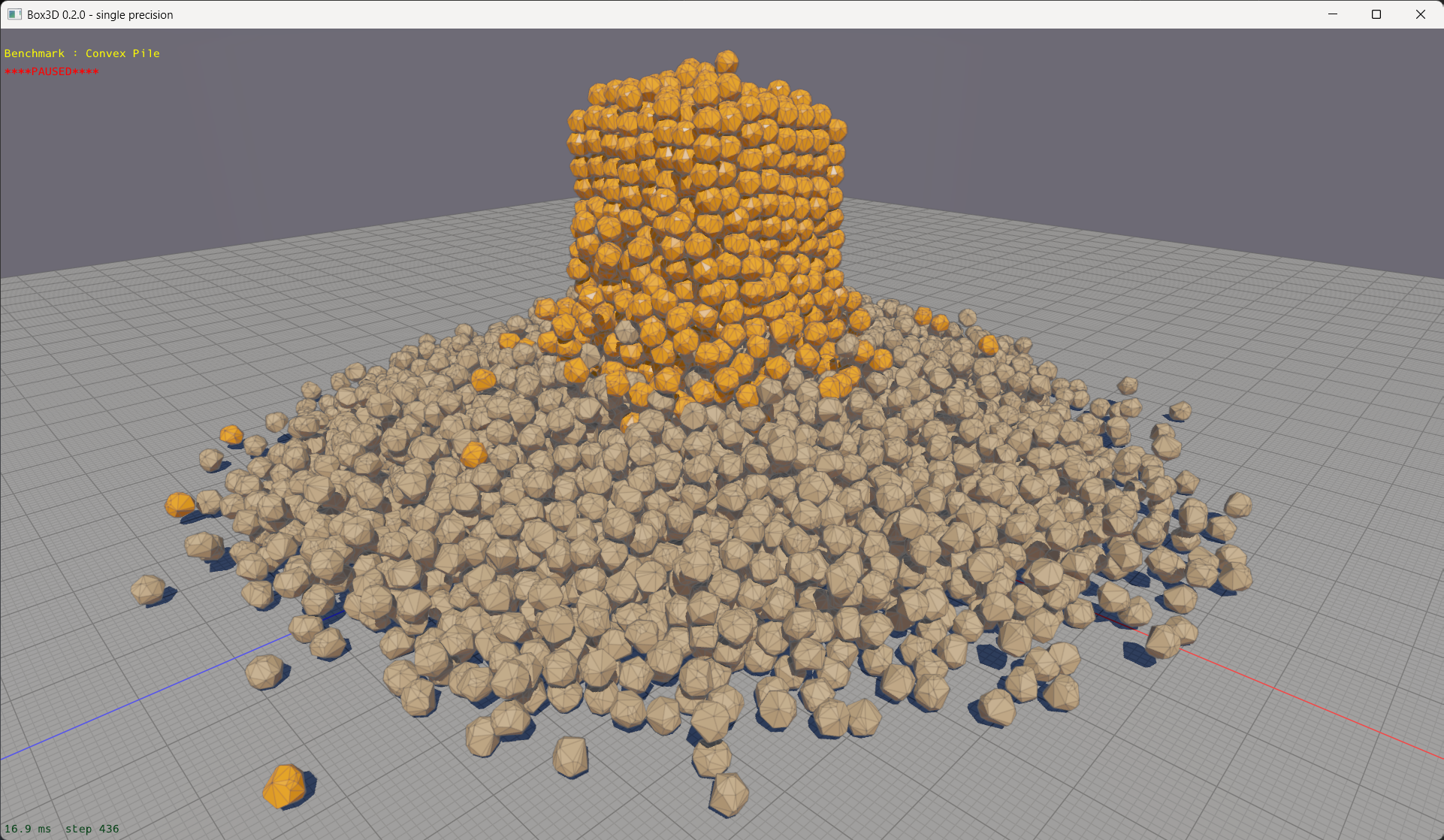 Convex Pile
Inscribed sphere technique
In 2011 the illustrious Pierre Terdiman suggested using internal objects to speed up SAT. The main idea is to use inscribed spheres to compute a cheap upper bound on the separation achievable by every face and every edge pair. The work described here goes further than what Pierre documented. The headline is that I have developed a scheme to use the Gauss map edge arc to cull edges before they even reach the edge pair test. Before I get to that, let’s warm up by looking at 2D.
Consider the 2D case with convex polygons and inscribed circles.
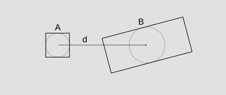 Boxes with inscribed circles
The vector \(d\) connects the centers of the two circles inscribed in A and B. The key observation is that the separation between the boxes is never more than:
$$\|d\| - (r_A + r_B)$$This means no separating axis can achieve a separation greater than this. This is the separation upper bound. The following figure shows an example axis \(n\). The actual separation \(\text{sep}(n)\) is clearly less than the bound.
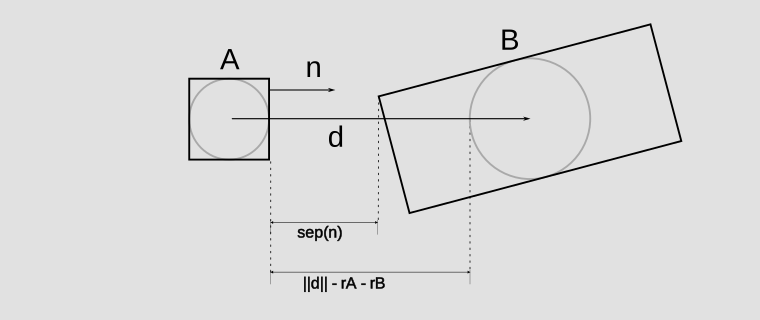 Example axis
Let’s remove the boxes and focus on the circles. Then I’ll combine the circles using the standard Minkowski equivalence. So we are looking at the separation between a circle and a point.
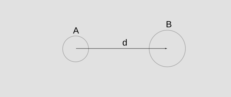 Inscribed circles
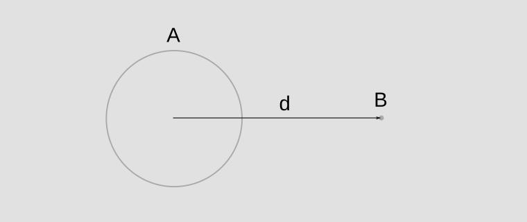 Minkowski conversion to circle and point
This all seems pretty basic. But now consider any candidate unit length separating axis \(n\) coming out of \(A\). The upper bound on the separation is:
$$n \cdot d - r$$where \(r = r_A + r_B\). This bound is better because it is tighter than the first bound using \(\|d\|\) and requires just a single dot product. Note that normals on polygon B require using \(-d\) in the bound.
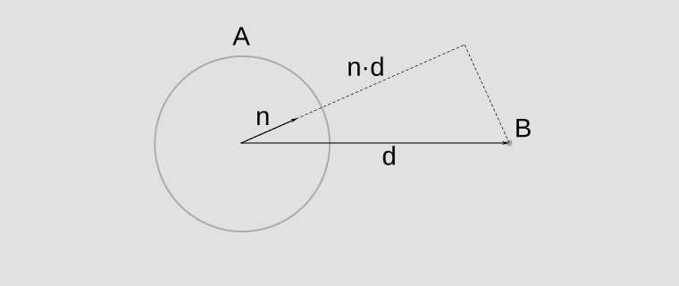 Candidate axis n
Keep in mind that this bound is not the escape distance. It is a bound on what the SAT can compute for the axis \(n\). The escape distance can be smaller. Consider a point in a unit circle at \([1/2, 0]\). Then \(d = [1/2, 0]\). In the +y normal direction the upper bound separation computed is:
$$n \cdot d - r = [0, 1] \cdot [1/2, 0] - 1 = -1$$The separation is -1, so the overlap value is +1. The escape distance \(q\) is smaller, around 0.866. But this is fine. SAT doesn’t give us the escape distance in every direction. It projects shapes along an axis and finds the overlap of the intervals. The inscribed circle technique gives us an upper bound on separation of the projected intervals.
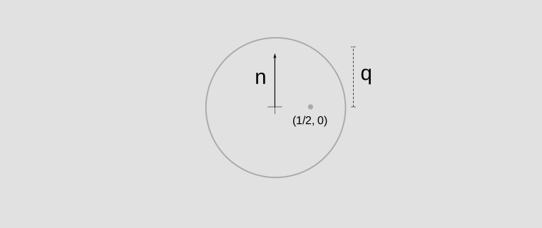 Escape distance
This is also not a local search technique. SAT is inherently a non-convex optimization problem when shapes overlap, so a local search can get stuck in a local maximum. The inscribed circle technique is still doing a global search.
So how does this help? Here’s the baseline separating axis test for the faces of A:
int bestIndex = -1;
float maxSeparation = -FLT_MAX;
for (int i = 0; i < countA; ++i)
{
  // Normal and point for face on polygon A.
  Vec nA = nAs[i];
  Vec vA = vAs[i];

  // Find deepest vertex on polygon B along normal.
  float si = FLT_MAX;
  for (int j = 0; j < countB; ++j)
  {
    float sij = Dot(nA, vBs[j] - vA);
    if (sij < si)
    {
      si = sij;
    }
  }

  if (si > maxSeparation)
  {
    maxSeparation = si;
    bestIndex = i;
  }
}
If both polygons have \(N\) points then this computation is \(O(N^2)\). Using the inscribed circle bound this can be re-written as:
int bestIndex = -1;
float maxSeparation = -FLT_MAX;
for (int i = 0; i < countA; ++i)
{
  // Normal and point for face on polygon A.
  Vec nA = nAs[i];

  // Skip this face if it can't beat the current maximum.
  if (Dot(nA, d) - r < maxSeparation)
  {
    continue;
  }

  Vec vA = vAs[i];

  // Find deepest vertex on polygon B along normal.
  float si = FLT_MAX;
  for (int j = 0; j < countB; ++j)
  {
    float sij = Dot(nA, vBs[j] - vA);
    if (sij < si)
    {
      si = sij;
    }
  }

  if (si > maxSeparation)
  {
    maxSeparation = si;
    bestIndex = i;
  }
}
This on its own is quite amazing because it can trade \(N\) dot products for one. Since this culling is desirable, it is helpful to seed the initial maximum with the separation along the face most aligned with \(d\). For polytope B I test the faces seeded with the face most aligned with \(-d\), accounting for the maximum separation from polytope A.
Note the value of \(r\) used above should be reduced slightly to protect against round-off problems. I use a combination of a relative and absolute tolerances (in meters).
$$r = r_0 - (0.005 + 0.001 (\|d\| + r_0))$$Edge culling
Speeding up the face tests is nice, but the elephant in the room is the 3D edge pair tests needed for colliding polytopes. The inscribed sphere test can be used to completely rule out an edge of a polytope for consideration before it even reaches the pair test. This way we can vastly reduce the number of pairs tested.
The Gauss map for a polytope represents faces as vertices on a unit sphere. Edges become arcs joining those vertices. When hulls collide the Minkowski difference combines those Gauss maps (B is negated). When arcs from polytope A intersect arcs from polytope B a vertex is generated on the Gauss map and this represents a face of the Minkowski difference. This face has a normal that is in the range of both Gauss map arcs.
For a given edge we know any separating axis it generates will be somewhere along its Gauss map arc, which is defined by sweeping the normal between the two adjacent faces. The image below shows this arc in a top down view of the edge. The vector \(w\) is the projection of \(d\) into the plane spanned by \(n_1\) and \(n_2\) (perpendicular to the edge).
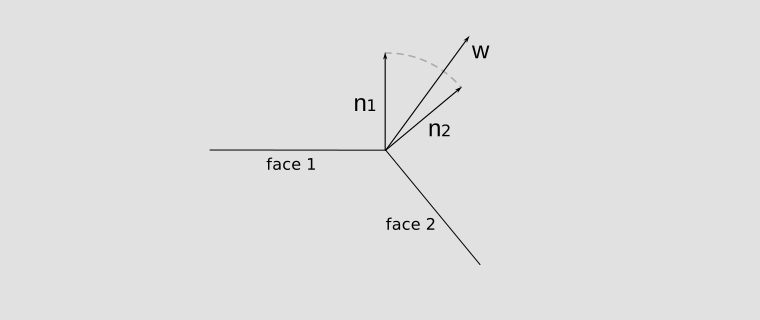 Gauss arc for an edge
If \(w\) is between the face normals then the upper bound separation is:
$$\|w\| - r$$If this bound exceeds the maximum face separation then this edge is a candidate for the edge pair test. If \(w\) is outside the arc then the edge bound is capped by the upper bound of the adjacent faces:
$$\max(n_1 \cdot d, n_2 \cdot d) - r$$An edge can still form the maximum separating axis when \(w\) is outside the arc, as long as the upper bound exceeds the maximum face separation.
The math for finding the edge upper bound separation is conceptually simple but a careful implementation can yield significant performance gains. Another thing to consider is that culling edges does not involve updating the current maximum separation. That comes later when edge pairs are considered. All we want is a yes/no result: is this edge a candidate for the edge pair stage?
I’ve already put a lot of detailed comments in the Box3D code for this. So I’ll just put the whole thing here so you don’t need to dig through the code. Note that when testing hull B the direction \(d\) must be flipped.
// A hull edge is bounded by two face normals. On the Gauss map the edge becomes an arc between
// those two face normals. An edge can only build the best separating axis if a normal on that arc
// can beat the best separation value seen so far. This function determines if the upper bound
// separation on that arc can possibly beat the current maximum face separation.
//
// This follows the upper bound used for hull faces:
// separation_upper_bound = dot(axis, centerB - centerA) - innerRadiusA - innerRadiusB
//
// Define:
// d = centerB - centerA
//
// Inputs:
// a1 = dot(n1, d)
// a2 = dot(n2, d)
// c = dot(n1, n2)
// bound = maxFaceSeparation + radiusBound
//
// This returns 1 if the edge is a candidate and 0 otherwise.
static inline int b3TestEdgeCandidate( float a1, float a2, float c, float bound )
{
  // c = cos(theta), the angle between the normals.
  // s = sin(theta)^2 >= 0
  float s = 1.0f - c * c;

  // This is coincidentally the law of cosines. Break out your protractor.
  float t = a1 * a1 + a2 * a2 - 2.0f * a1 * a2 * c;

  // Exterior conditions:
  // Can either face normal beat the best separation? These cover the case where d
  // is outside the arc wedge. Note that d pointing outside the arc wedge does not cull
  // this edge. It can still generate the maximum separation (which happens commonly).
  int exterior = b3MaxFloat( a1, a2 ) >= bound;

  // Project d into the plane that holds both n1 and n2, call that vector w.
  // Introduce the coordinates b1 and b2 (these have units of length).
  //
  // w = b1*n1 + b2*n2
  //
  // Since w is the projection of d into the plane spanned by n1 and n2:
  // dot(n1, w) == dot(n1, d) == a1
  // dot(n2, w) == dot(n2, d) == a2
  //
  // Dot the equation with n1 and n2:
  // a1 = b1 + b2*c
  // a2 = b1*c + b2
  //
  // Solve for b1 and b2 using Cramer's Rule
  // b1 = (a1 - a2 * c) / s
  // b2 = (a2 - a1 * c) / s
  //
  // s = 1 - c * c is positive, so b1 and b2 must be positive for w to live in
  // the arc between n1 and n2.
  //
  // The peak value of dot(n, d) on the arc is then norm(w):
  // dot(w, w) = dot(b1*n1 + b2*n2, d)
  //           = b1*a1 + b2*a2
  //           = (a1*a1 - a1*a2*c + a2*a2 - a1*a2*c) / s
  //           = (a1*a1 + a2*a2 - 2*a1*a2*c) / s
  //           = t / s
  //
  // The interior is a candidate if:
  // norm(w) >= bound
  // sqrt(t / s) >= bound
  // If bound < 0 this is always true. Otherwise
  // t >= bound^2 * s
  //
  // Interior conditions:
  // b1 and b2 positive (interior arc): a1 >= c * a2 & a2 >= c * a1
  // bound <= 0.0: the interior arc is automatically a candidate because it is positive
  // s < B3_PARALLEL_TOL : n1 and n2 are nearly parallel so give up and pass the edge to the next stage
  // t >= bound * bound * s : bound is positive and the interior normal direction is a candidate
  //
  // Using bit ops here to avoid branches.

  int interior =  ( a1 >= c * a2 ) & ( a2 >= c * a1 ) &
                  ( ( bound <= 0.0f ) |
                  ( s < B3_PARALLEL_TOL ) |
                  ( t >= bound * bound * s ) );

  return exterior | interior;
}
Results
There is a Hull Culling sample in Box3D that shows the culling results for a pair of hulls from the Convex Pile sample.
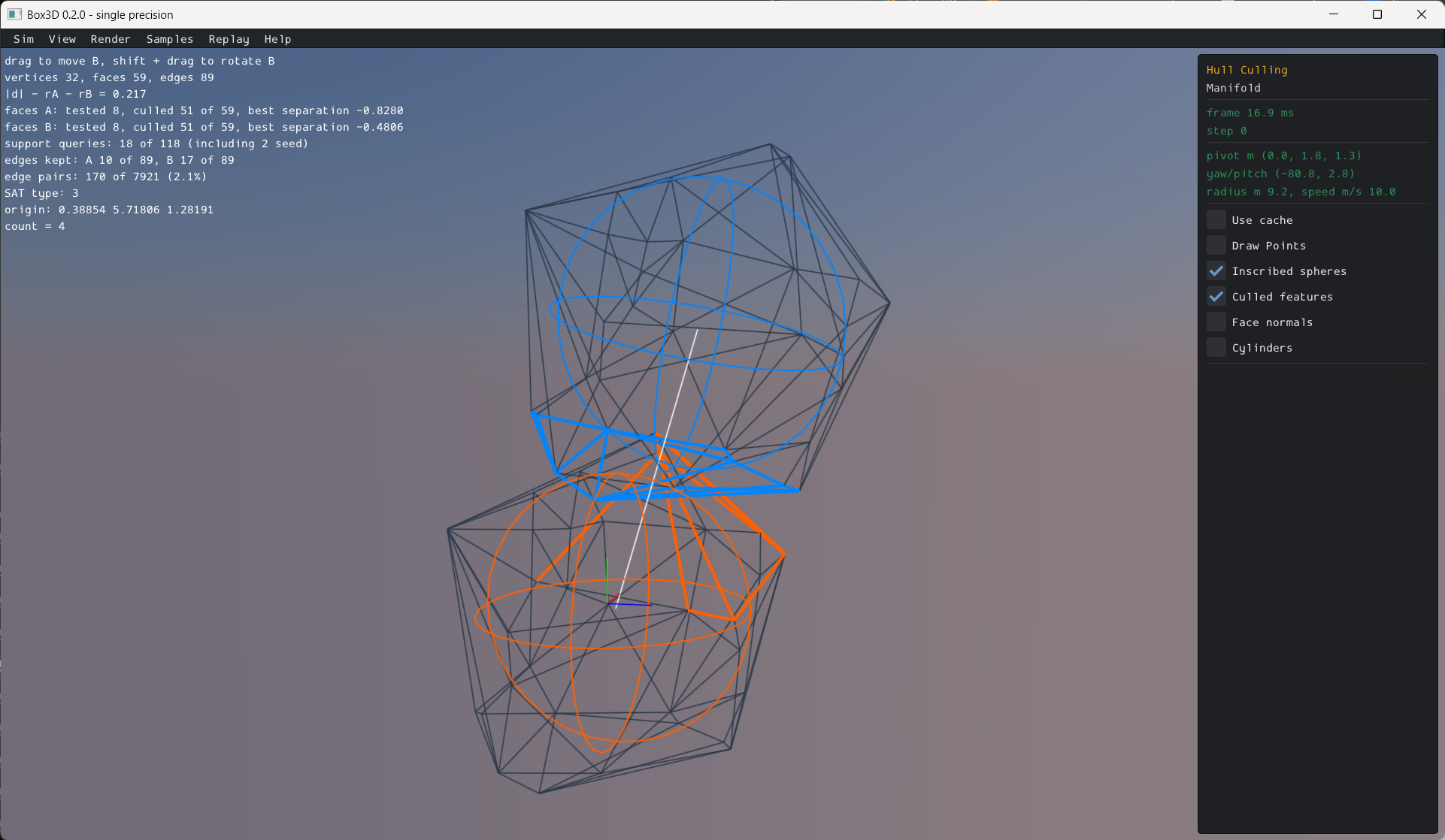 Hull culling
Each hull has 32 vertices, 59 faces, and 89 edges. Typically games can get away with simpler hulls, so these hulls are a good stress test for the narrow-phase (collide in the benchmark table below).
For the configuration shown 86% of the face tests are culled and 98% of the edge pair tests are culled. This results in a dramatic speed up of SAT. The Convex Pile benchmark roughly doubled in performance, meaning the narrow-phase more than doubled in performance.
I’m guessing you are curious about other less sphere-like shapes. So I tested two skinny cylinders, each with 64 vertices. The relatively small inscribed spheres lead to less culling. In this case 76% of the edge pairs get culled. This is somewhat like back-face culling. If we can cull 50% of the edges from a hull then the number of pairs is reduced by 75%.
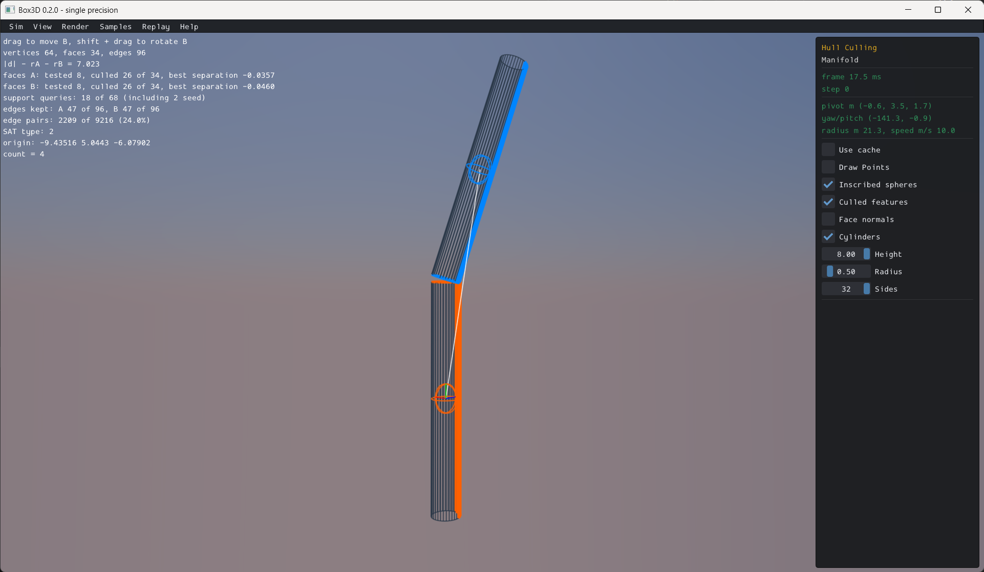 Cylinder culling
And when does culling completely fail? When shapes are deeply overlapped almost nothing is culled. Deep overlap rarely happens in games and it is usually short lived.
I ran benchmark deltas with and without the inscribed sphere cull. These have progressively more complex hulls. The washer benchmark shows a gain for box hulls so there is no regression on simple hulls. Junkyard uses a 10 point rock shaped hull and shows a solid gain. And finally the Convex Pile shows the top gain. I’ve included the other stages to indicate the level of noise in the benchmarks and to provide perspective on the relative costs of each stage. The millisecond timing values here are for the full run: washer runs 1000 steps, junkyard 500, and convex_pile 500.
| Benchmark | Stage | Before (ms) | After (ms) | Change |
|---|---|---|---|---|
| washer | pairs | 481.2 | 483.5 | +0.5% |
| collide | 2,191.5 | 2,034.8 | -7.1% | |
| solve | 1,892.0 | 1,892.5 | 0.0% | |
| total | 4,573.9 | 4,431.1 | -3.1% | |
| junkyard | pairs | 257.5 | 266.5 | +3.5% |
| collide | 1,699.5 | 1,473.6 | -13.3% | |
| solve | 1,037.2 | 1,031.2 | -0.6% | |
| total | 3,003.9 | 2,779.2 | -7.5% | |
| convex_pile | pairs | 178.0 | 173.7 | -2.4% |
| collide | 2,567.6 | 976.7 | -62.0% | |
| solve | 360.0 | 357.3 | -0.7% | |
| total | 3,109.4 | 1,512.3 | -51.4% |
Now let’s compare the performance of SAT versus GJK. I benchmarked SAT and GJK for combinations of three shapes: complex (32 pt), rock (10 pt), and cylinder (64 pt).
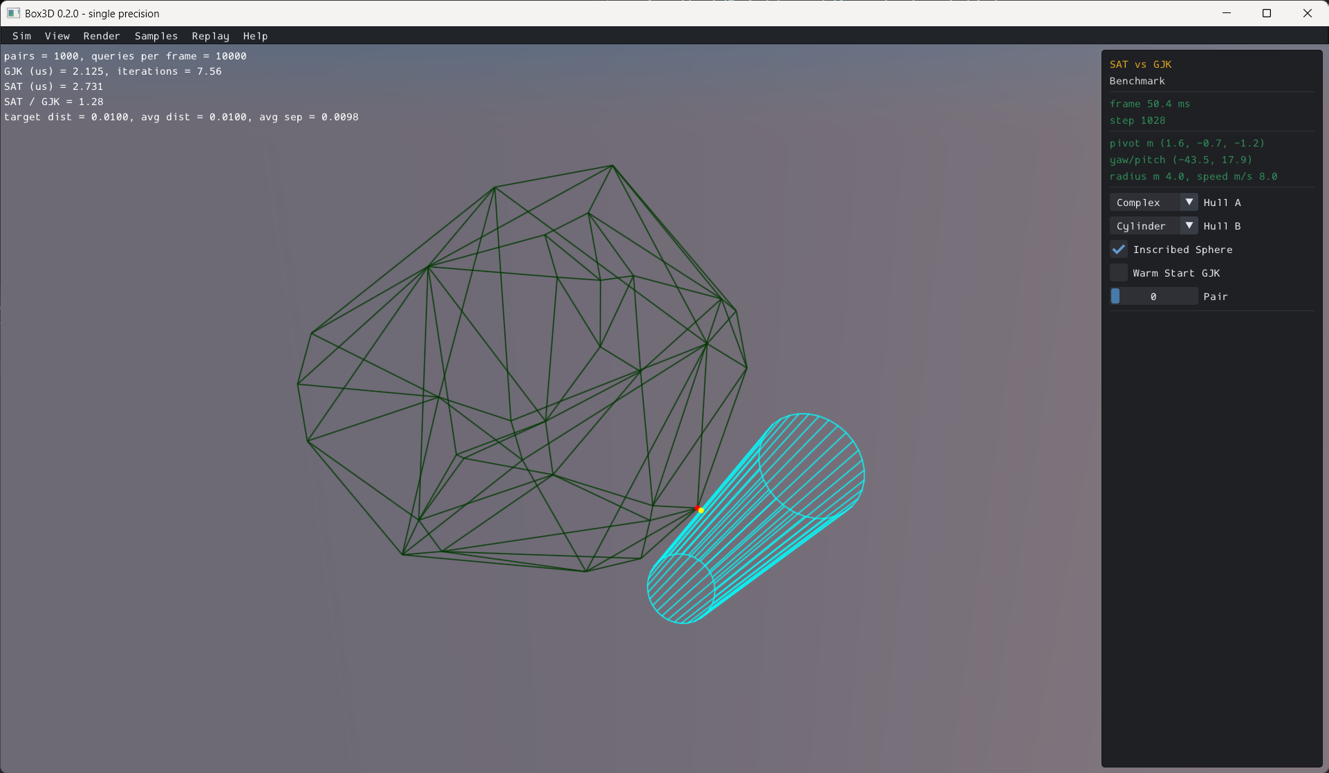 SAT versus GJK
GJK handles distance better than SAT while SAT handles overlap better than GJK. So I setup the benchmark carefully to make a fair comparison. Each configuration is built by randomly rotating and positioning the second hull then using the shape distance to slide it to about 1cm of distance. This is within the Box3D speculative band, so it is a realistic scenario. In this regime SAT and GJK have no early outs.
Here is the table of results. Timings are the average microseconds per call over thousands of random configurations. For SAT this only includes the cost of finding the maximum separating axis and the separation value. For GJK the cost only includes computing the distance and the closest points. No contact points are computed in either case. No caching or warm starting is used.
| Hull pair | GJK | SAT | SAT (no sphere bound) | SAT / GJK | Sphere bound speedup |
|---|---|---|---|---|---|
| complex / complex | 1.29 | 1.65 | 10.64 | 1.27× | 6.4× |
| complex / rock | 0.98 | 1.01 | 4.37 | 1.03× | 4.3× |
| complex / cylinder | 2.02 | 2.56 | 10.75 | 1.27× | 4.2× |
| rock / rock | 0.53 | 0.44 | 1.66 | 0.84× | 3.7× |
| rock / cylinder | 1.59 | 1.60 | 4.69 | 1.01× | 2.9× |
| cylinder / cylinder | 2.45 | 5.74 | 13.26 | 2.34× | 2.3× |
This shows that SAT with the inscribed sphere and SIMD optimizations is finally competitive with GJK. Long skinny shapes, such as the cylinder, are still a challenge for SAT, but Dirk has some ideas that might help (see below).
Summary
Edge culling using inscribed spheres makes SAT significantly faster for hulls with many edges. This technique gives the global maximum separation value. It is not approximate and cannot get stuck in a local maximum. It is a simple addition to the SAT algorithm. You can bolt this culling approach into your code using a couple of small functions and get large performance gains for complex hulls.
The main pipeline requirement is to compute the inscribed sphere. This doesn’t have to be optimal. Box3D just computes the hull centroid and then finds the closest face plane to determine the radius. Just an \(O(N)\) scan while the hull is being built. This turns out to be generally useful and I already use the inscribed sphere for CCD.
References
Pierre’s article is the inspiration for the inscribed sphere technique. Choi provides the fast edge pair Minkowski test popularized by Dirk. Cairn sketched the SIMD edge pair test in Box3D. The last three provide detailed explanations of the Gauss map.
- Pierre Terdiman: Faster convex-convex SAT: internal objects
- Choi et al.: Computing the Minimum Directional Distance between Two Convex Polyhedra
- Dirk Gregorius: The Separating Axis Test between Convex Polyhedra
- Cairn Overturf: Improvements to the Separating Axis Test
Addendum
Cairn suggests deriving the edge upper bound using a function maximum found through differentiation. This gives a different perspective than the geometric approach above and may be more efficient.
Dirk suggests using the polytope border when computing the upper bound for an edge. The other polytope is still represented by its inscribed sphere. This should be better for long shapes where the inscribed sphere is relatively small.