SIMD for Collision
In a previous post SIMD Matters I discussed the big wins I got from graph coloring to make the contact solver faster. That same approach exists in Box3D. I like to call this approach “wide SIMD”. The idea is to process multiple work units at the same time. In the contact solver this means solving four contact points at the same time.
This is different from “narrow SIMD” where a 3-vector (xyz) is put into a SIMD register and then standard vector math is expressed as SIMD intrinsics. Narrow SIMD can be useful, but the gains are not as obvious.
In 3D there is an opportunity for using wide SIMD that doesn’t exist in 2D. Consider the convex pile benchmark ported from PEEL. This benchmark drops 5120 convex hulls, each with 32 points.
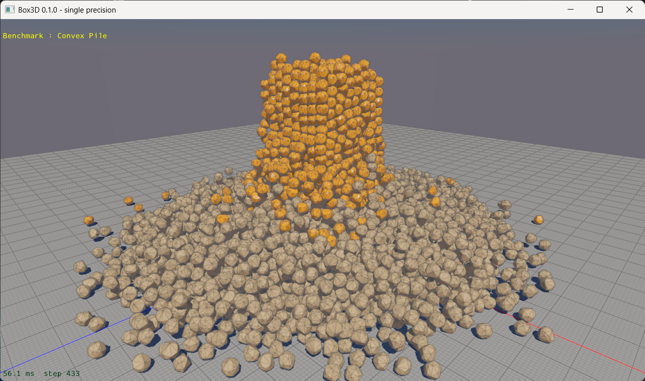
Box3D treats boxes as hulls and many of the benchmarks use boxes. The performance with boxes has been good and typically most of the cost is not in the narrow phase. But the 32 point hull is a different beast. Let’s call it “boulder”. The table below shows the hull details for a box compared to the boulder.
| Hull | Vertices | Faces | Edges |
|---|---|---|---|
| Box | 8 | 6 | 12 |
| Boulder | 32 | 59 | 89 |
Box3D uses the Separating Axis Test for collision detection. This is abbreviated as SAT. Using SAT I can find the best features to use for pushing the shapes apart and precisely how far apart they need to be pushed to remove overlap. Furthermore, I use these results to compute the contact normal and the contact points.
Other physics engines may use the distance algorithm GJK instead with an overlap fallback such as the Expanding Polytope Algorithm, also known as EPA.
I’m a big fan of SAT for convex hull collision because it doesn’t require a collision margin. Shapes can rest directly on each other. The GJK and EPA combo usually tries to keep shapes slightly separated to stay in the GJK region, which is faster. This can lead to visual gaps. Also, EPA can be numerically brittle and often physics engines will need a fallback if EPA fails: a fallback for the fallback. EPA is essentially an algorithm for computing a convex hull, and the input data can be flat slivers. That is a challenging scenario for convex hull computation. Hence the need for a second fallback.
Unfortunately, SAT in 3D has quadratic complexity. With two hulls A and B, the collision algorithm must test the faces of hull A against the vertices of hull B, the faces of hull B against the vertices of hull A, and the edges of hull A against the edges of hull B. In the worst case, every combination must be evaluated.
| Combination | Face-Vertex | Vertex-Face | Edge-Edge |
|---|---|---|---|
| Box-Box | 6 | 6 | 144 |
| Boulder-Boulder | 59 | 59 | 7921 |
The number of edge-edge combinations grows quadratically. There are some tricks to speed up the edge tests using the Gauss Map. See Improvements to the Separating Axis Test for more details. Regardless, the edge-edge test can easily dominate the entire simulation.
So what does this edge-edge code look like? At a basic level it looks like this:
for (Edge edgeA : hullA.edges)
{
    for (Edge edgeB : hullB.edges)
    {
        TestCrossProduct(edgeA, edgeB);
    }
}
If there are just 12 edges in each hull, doing SIMD on this is not a big win because SIMD requires some setup work. For SIMD to work well the data needs to be in structure of arrays format (SoA).
With 89 edges in each hull the story changes drastically. There are 7921 calls to TestCrossProduct. With wide SIMD I can test one edge of hullA against four edges of hullB simultaneously. It looks sort of like this:
for (Edge edgeA : hullA.edges)
{
    for (EdgeWide edgeWideB : hullB.edgesWide)
    {
        TestCrossProductWide(edgeA, edgeWideB);
    }
}
There are a lot of hidden details in the snippet and you can look at the Box3D code if you are curious. But I’m here to answer the question: should we care about SIMD for collision detection? Well, I have results! These are the results for the convex pile benchmark with the total milliseconds for a 500 step run. I tested 1 to 8 threads on an AMD 7950x with the CPU pegged at 4.42GHz. The results are the best of 4 runs.
| Threads | Scalar | SSE2 | AVX2-Lite |
|---|---|---|---|
| 1 | 40706 | 17337 | 15762 |
| 2 | 20799 | 8857 | 8131 |
| 3 | 13789 | 5946 | 5471 |
| 4 | 10324 | 4509 | 4084 |
| 5 | 8359 | 3675 | 3361 |
| 6 | 6958 | 3106 | 2843 |
| 7 | 6006 | 2697 | 2477 |
| 8 | 5292 | 2410 | 2277 |
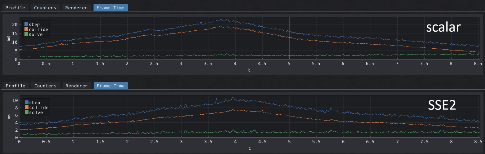
SSE2 is over twice as fast as scalar! Keep in mind these timings are for the entire simulation, not just the edge-edge test. The scalar column also indicates that the contact solver runs in scalar mode. So this is the full picture of the simulation.
Box3D only implements SSE2 intrinsics. In Box2D I have AVX2 intrinsics as well, but there were a surprising number of users without AVX2 capable CPUs. Nevertheless, just enabling the AVX2 architecture in Box3D gives a nice gain, as indicated in the AVX2-Lite column. Free performance gains are great to see. In the future I may try a real AVX2 implementation testing 8 edges at a time.
This benchmark represents a 32-point hull with 89 edges. Surely SAT will be overrun as the point count grows further. Well, fortunately Box3D has a hard 128 edge limit. This limit already existed and has to do with keeping the hull storage compact (8-bit indices and two half-edges per edge). Somewhat surprisingly, converting complex hulls to meshes can solve the quadratic growth problem, but it makes the shape less suitable for a dynamic body.
You may wonder if the SIMD edge tests moved the needle on box-box. Sadly it has almost no effect. This optimization seems to only benefit complex hulls. Such hulls can come up in several scenarios, such as destruction. So it is a worthy addition to Box3D.
Finally, here is a video comparison and a side-by-side of the frame timings.