SIMD Matters
SIMD in game development
Often in game development we talk about SIMD. It is the holy grail of CPU performance, often out of reach. The conventional wisdom is that it is difficult to achieve real gains from SIMD.
It is tempting to build a math library around SIMD hoping to get some performance gains. However, it often has no proven benefit. It just feels good to be using something we know can improve performance. But sometimes SIMD can get in the way.
For example, game play programmers often do a lot of piecemeal vector math. They are not chopping 8 carrots at once. Instead they are trying to get a movement ability to work well on the player. Like swinging on a rope or swimming in water. These require vector math, but this code cannot be gathered into SIMD instructions in a meaningful way. We cannot force a game to have 8 players swinging on a rope at the same time.
Game physics is often similar. The user wants to create or destroy a single body. The ray casts are issued from the game separately and point in different directions.
Even if there are many similar things being computed, it can be difficult to gather these objects and push them through some algorithm simultaneously. For example, in game physics one of the most expensive computations is computing the contact forces between colliding bodies. When there are many bodies there can be a huge number of contact points.
This large pyramid has 5050 bodies and a whopping 14950 contact pairs, each with two contact points. Each contact point has a non-penetration force and a friction force. That is 59800 forces to be computed! Further these forces need to be computed several times per time step as part of the Soft Step solver. Read more here.
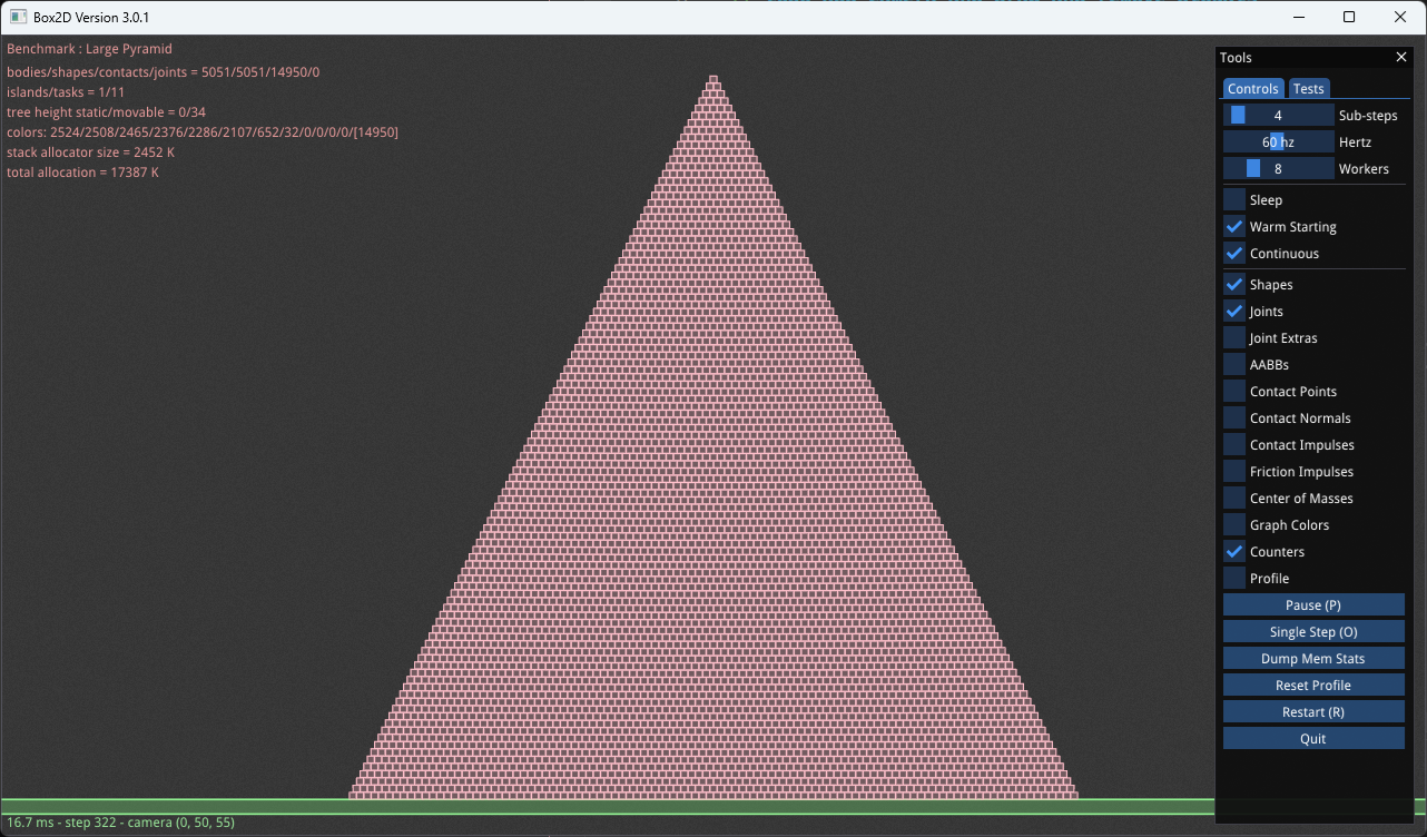 A pyramid of 5050 bodies
Another problem is that each constraint operates on different bodies. So even if constraints are organized contiguously in an array for faster iteration, the bodies need to be randomly accessed. This random access is the ultimately the bottleneck in game physics.
Graph coloring
For Box2D version 3.0 I decided to finally try using SIMD as it is meant to be used for solving contacts. Making contacts solve faster could yield large performance gains so I decided it would be worth the effort.
But how can I gather 4 or 8 contact pairs to be solved simultaneously? The key is graph coloring. The idea is to have a handful of colors to be assigned to all the contact constraints. For example, suppose I have 6 colors and I want to assign all the contacts to one of those 6 colors. Contact constraints act upon two bodies at a time. With graph coloring the restriction is that within a single color a body can only appear once or not at all.
This small pyramid shows an example of graph coloring. Each contact constraint has two contact points with the same color. There are four colors: red, orange, yellow, and green. If you look at a color, such as orange, you can see that it only touches a box once per contact point pair. This is the magic of graph coloring and enables me to solve multiple contact constraints simultaneously without a race condition.
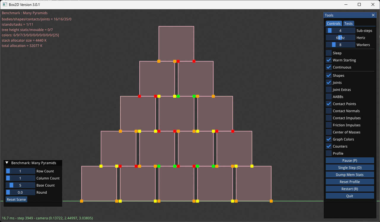 Graph coloring of a small pyramid
Graph coloring can scale to very large scenarios. The image below shows the graph coloring of the contact points on the large pyramid. You can see in the text the number of contact constraints per color.
- color 1 : 2524
- color 2 : 2508
- color 3 : 2465
- color 4 : 2376
- color 5 : 2286
- color 6 : 2107
- color 7 : 652
- color 8 : 32
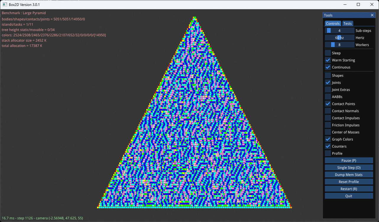 Graph coloring of the large pyramid
These colors group together constraints that can be solved simultaneously using SIMD. For example, color 1 has 2524 contact constraints. Each of these constraints is between two bodies. The graph coloring ensures that none of the same bodies appear more than once in all 2524 contact constraints. This means all 2524 constraints can be solved simultaneously.
But isn’t graph coloring very complex and slow? Contacts come and go all the time in rigid body simulation. Do I need to recompute the graph colors every time a contact is added or removed?
First of all, there is a lot of intimidating theory around graph coloring and it seems at first that some complex algorithms must be applied to do graph color properly. This is not true at all! A simple greedy algorithm is sufficient for game physics.
Box2D maintains a bitsets for each graph color. Each bit corresponds to a body index. When a contact constraint is created, the graph color bitsets are examined. The constraint is assigned to the first color with a bitset that doesn’t have either body bit set to 1. Once the constraint is assigned to a color, those two body bits are set to 1. This is a very fast operation.
void b2AddContactToGraph(b2ConstraintGraph* graph, b2Contact* contact)
{
    int indexA = contact->bodyIndexA;
    int indexB = contact->bodyIndexB;

    for (int i = 0; i < graph->colorCount; ++i)
    {
        b2GraphColor* color = graph->color + i;
        if (b2GetBit(color->bodySet, indexA))
        {
            // advance to next color
            continue;
        }

        if (b2GetBit(color->bodySet, indexB))
        {
            // advance to next color
            continue;
        }

        // available color found!
        b2SetBit(color->bodySet, indexA);
        b2SetBit(color->bodySet, indexB);

        contact->colorIndex = i;
    }
}
Even though bitsets are fast, it would be better not to redo the graph coloring every time step. So Box2D persists the graph coloring across time steps. When a contact constraint is created the color is determined and the body bits are turned on. When a constraint is removed the corresponding two body bits are cleared.
void b2RemoveContactFromGraph(b2ConstraintGraph* graph, b2Contact* contact)
{
    b2GraphColor* color = graph->color + contact->colorIndex;
    b2ClearBit(color->bodySet, contact->bodyIndexA);
    b2ClearBit(color->bodySet, contact->bodyIndexB);
    contact->colorIndex = B2_NULL_INDEX;
}
There are a couple more details. When bodies go to sleep they are removed from the graph coloring and when they wake they are added back according to the constraints that connect them. Also static bodies are never set in the bitsets because static bodies are not modified by the contact solver. This reduces the number of colors needed.
Going WIDE
So now that I have 2524 contact constraints I can solve simultaneously, how do I do that? Well there are no SIMD units that are 2524 floats wide. So I break these into 4 or 8 constraint blocks (SSE2/Neon or AVX2). These wide constraints can be solved like a single scalar constraint. The math looks almost identical.
There is some delicate plumbing needed to make this happen. In particular, I need to gather 4 or 8 pairs of bodies for each wide constraint. I gather the body velocities and put them in wide floats (4 or 8 floats).
// wide float
typedef b2FloatW __m128;

// wide vector
struct b2Vec2W
{
    b2FloatW X;
    b2FloatW Y;
};

// wide body
struct b2BodyW
{
    b2Vec2W linearVelocity;
    b2FloatW angularVelocity;
};
I grab 4 or 8 bodies and stuff their velocities into a single wide body. Then the wide constraint operates on wide bodies and all the math looks similar to scalar math. For example, the wide dot product is just two multiplications and one addition, doing 4 or 8 dot products simultaneously.
// wide dot product
b2FloatW b2DotW(b2Vec2W a, b2Vec2W b)
{
    return b2AddW(b2MulW(a.X, b.X), b2MulW(a.Y, b.Y));
}
This is the way SIMD is meant to be used. But there is sure a lot of setup work to make this possible!
After the wide constraint is solved, the wide body velocities are scattered to the individual scalar bodies. These gather/scatter operations are needed to make this all work. Each instruction set SSE2/Neon/AVX2 has custom instructions that help with this. None of it is super intuitive but it is well documented not too difficult to setup.
Does it matter?
I did all this work to enable SIMD processing. Did it help? Box2D has a benchmarking console application to help answer this question. I implemented SSE2, Neon, and AVX SIMD instruction sets in the Box2D contact solver. I also implemented a scalar reference implementation. I have 5 benchmarks scenarios that push Box2D in various ways. See the benchmark results here.
I ran these benchmarks on an AMD 7950X (AVX2, SSE2, scalar) and an Apple M2 (Neon).
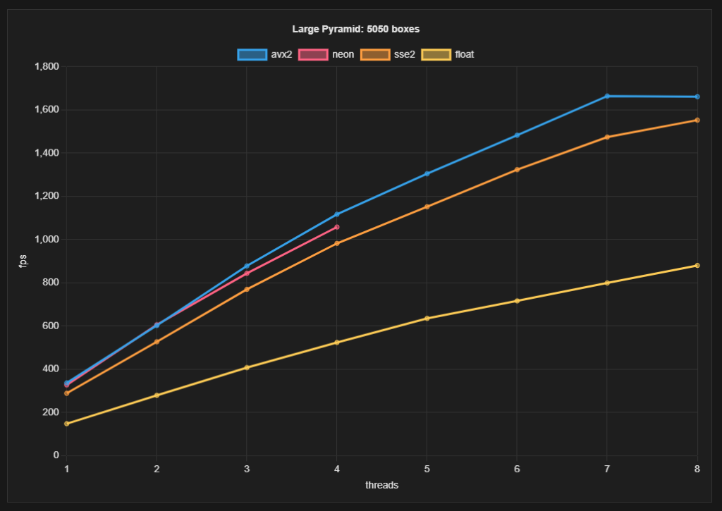 Large pyramid benchmark results
The joint grid benchmark doesn’t use SIMD instructions at all, so you can ignore that one. But the other ones all stress the contact solver.
The large pyramid benchmark with 4 workers has the following numbers:
- AVX2 : 1117 fps = 0.90 ms
- Neon : 1058 fps = 0.95 ms
- SSE2 : 982 fps = 1.02 ms
- scalar (AMD): 524 fps = 1.91 ms
- scalar (M2): 679 fps = 1.47 ms
From this I draw the following conclusions:
- SSE2 is about 2x faster than scalar
- AVX2 is about 14% faster than SSE2
- The Apple M2 smokes!
Another consideration is that all collision is done with scalar math. So more gains could be made if I figure out how to use SIMD for collision as well.
The bottom line is that making good use of SIMD can be a lot of work but it is worth the effort because it can make games run significantly faster and handle more rigid bodies.
What about compiler vectorization?
An interesting side result from this experiment relates to compiler vectorization. In my scalar reference implementation I defined the wide float as a structure of 4 floats.
// wide float for reference scalar implementation
struct b2FloatW { float x, y, z, w };
I also implemented all the wide math functions to work with this. It seems that I have arranged all the data perfectly for the compiler to use automatic vectorization. But it seems this doesn’t really happen to a sufficient degree to compete with my hand written SSE2. This is a bit ironic because on x64 all math is SIMD math, it is just inefficient SIMD math.
References
Bepu Physics uses graph coloring and SIMD. While I had known about this technique for some time, the high performance of Bepu has inspired me.
High-Performance Physical Simulations on Next-Generation Architecture with Many Cores. This is the earliest reference I know of that suggests using graph coloring to speed up rigid body physics calculations.
Graph coloring is used in many areas of simulation. For example, it is very useful for cloth simulation. The nice thing about cloth simulation is that typically the graph coloring can be pre-computed.
Update
- added milliseconds to comparison
- added M2 scalar results
1761 words
2024-08-18 17:00 -0700